Category: Filters (Page 1 of 2)

Low Pass Gate Emulation.

07/09/2025 / Stephen / 1 Comment

Post updated due to an error on my part when reading documents on the design of Buchla LPG module. 24/09/2025.

About Low Pass Gates (LPG).

What is a low pass gate, and how does it differ from a normal low pass filter, isn’t it the same item with a different name?
No It’s not. For a start the LPG doesn’t resonate in all modes. They were developed for the Buchla range of modular synthesizers, and have a more “acoustic” quality to them, think of the sound of a xylophone or bongos. Those instruments have a characteristic percussive and bright start to the sound, and the sound then quickly looses its brightness, and fades out slowly rather than dying away abruptly.
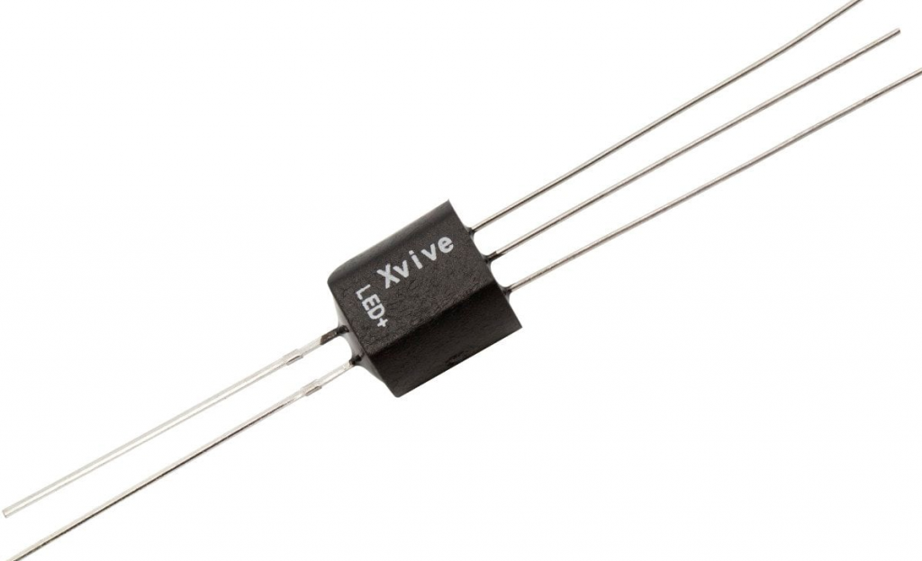
This was a result of using a rather unique method of applying voltage control to frequency and amplitude, this was done with a device known as a “Vactrol”, which was a combination of a light source (early devices used a filament lamp, later ones used LED’s) and a light sensitive resistor (LDR). Below are shown a VACTROL device, and (for those interested a VCA circuit using a VACTROL.

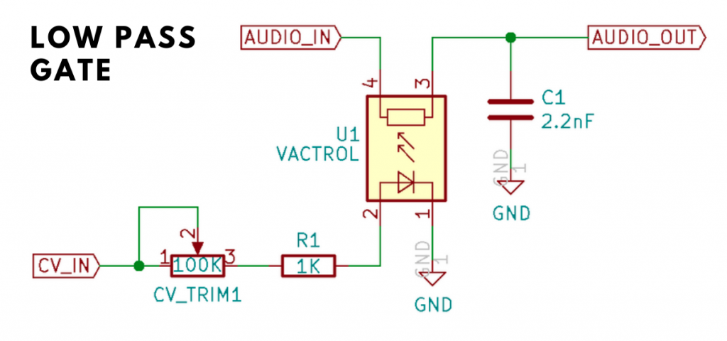
As the voltage supplied to the light source got brighter the resistance decreased thus changing the volume or cut-off frequency. Due to the nature of both these components, there was a varying lag between light brightness and the resistance of the LDR Both these devices are non-linear in their characteristics, which vary between devices. This means it’s not something you can emulate precisely
(it varied widely between modules-let alone synthesizers) , not that you need to as you’ll see later when we start putting our structure together.
Although there is non-linearity, and a lag between voltage variations and the effect on audio there is no inherent distortion in the LPG to take into account (unless it’s overdriven of course).

Note: This project uses Two of Elena Novaretti’s third party modules:
ED Exp, and ED Glider 2 (don’t use the Glider module, you can’t control the up/down times individually).

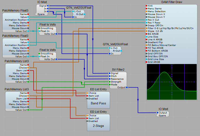
Generating the attack/decay envelope.

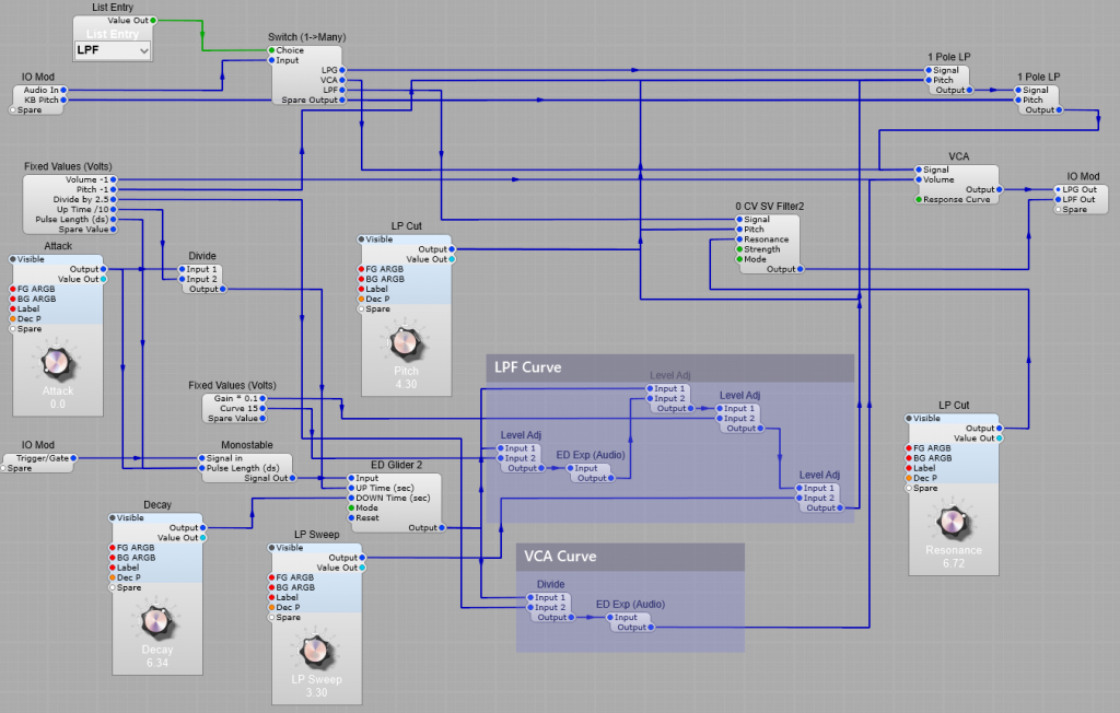
The Attack-Decal envelope for this project is different from the average ADSR envelope. We don’t need the Sustain and Decay portions of the envelope, just the attack and decay. You might think that having the the gate plug of the MIDI to CV2 module connected isn’t necessary, but I found that leaving the connection out caused some strange problems. For this reason I used a the Monostable to create a short pulse to trigger the ED Glider 2 module. One issue to take into account is that the ED Glider 2 module uses Volts per second for the Up and Down times, and the Monostable uses Volts per Deci-Second (10th’s of a second). For this reason I used a divider in the Rise time control line set to divide by 10 so that the Pulse out length from the monostable corresponds with the Up Time (Attack) of the Glide module. The pulse length needs to be the same as the Up Time for the Attack section of the envelope to work. The Down Time (Decay) portion of the envelope does not start until the input is at 0 volts. The Mode setting of the Glide 2 module should be left at the default Constant Time setting. The reset plug is not used.

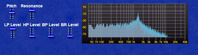
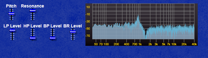
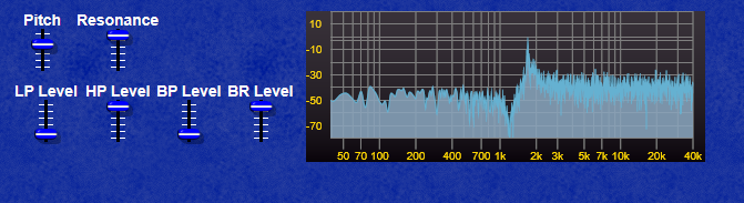
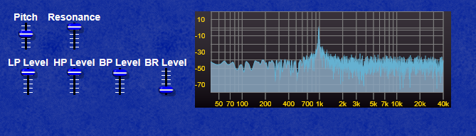
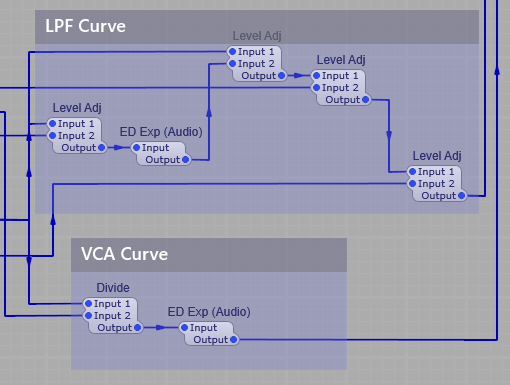
LPF Curve and VCA Curve.

You might think initially that having the two different methods of generating the curve for the envelope is a bit superflous, but I did this to imitate the effect that different Vactrol characteristics would have on the filter and VCA operation, so the envelope for the VCA is a straightforward exponential conversion, but the envelope for the Filter is quicker to decay meaning that when in the LPG option is selected the filtered sound will change in timbre more quickly than theloudness changes to give a more “percussive” sound to the output, where you get an initial bright start to the sound which then becomes naturally softer in timbre with the sound “ringing” on more than a conventional VCF/VCA combination.

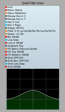
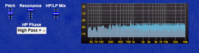
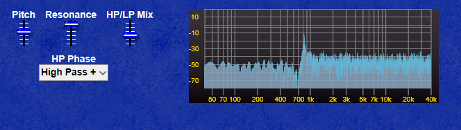
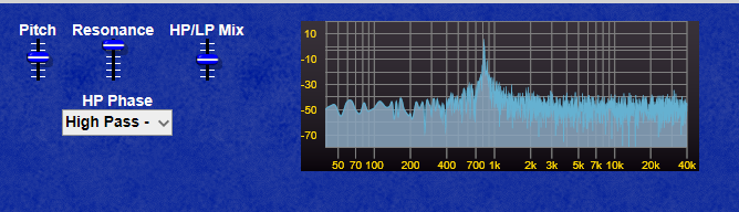
The screenshot below shows clearly how the CV curves for the LP Filter and the VCA differ in their curve, the LP Filter envelope decays quite quickly, whereas the VCA envelope has a far longer decay allowing the sound to “ring on” after the filter has reached it’s minum frequency (provided you leave the filter pitch at a point where the sound is still audible of course!)

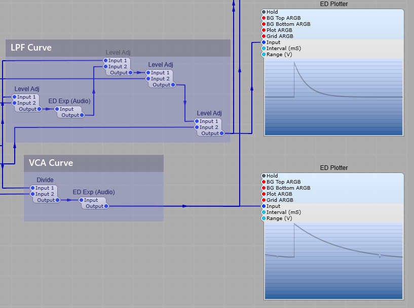
Note: If the CV for the filter exceeds 10 Volts, most filters will internally “clip” this voltage to prevent the filter module from misbehaving, however the VCA module will oveload with CV exceeding 10V and produce some very harsh sounding (and very loud) clipping.

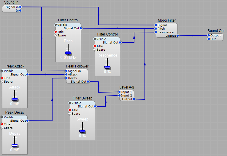
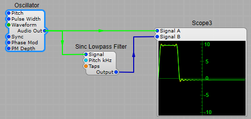
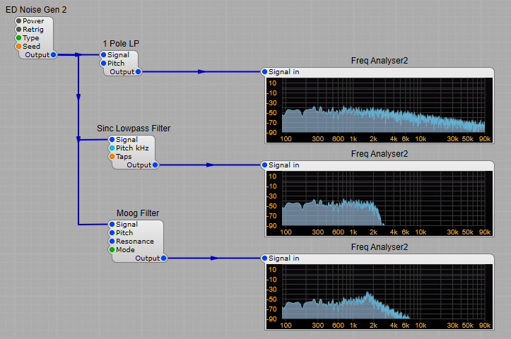
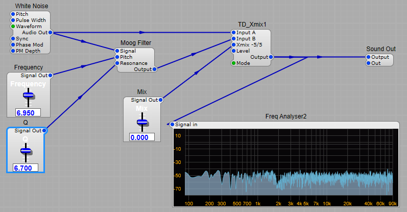
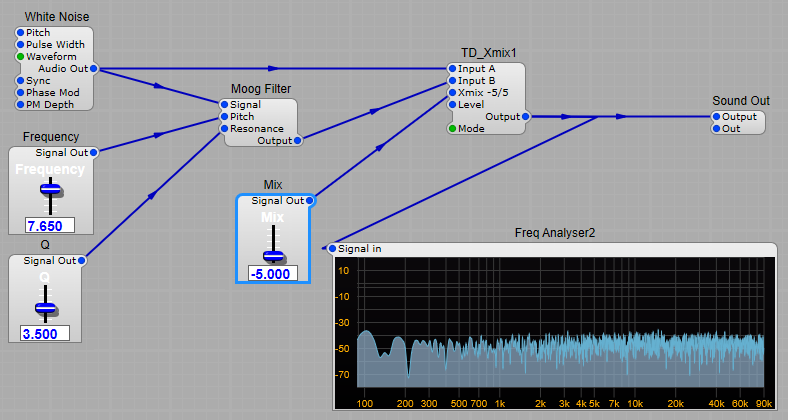
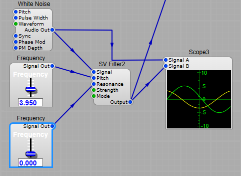
The filters

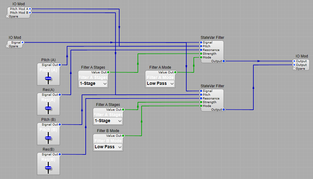
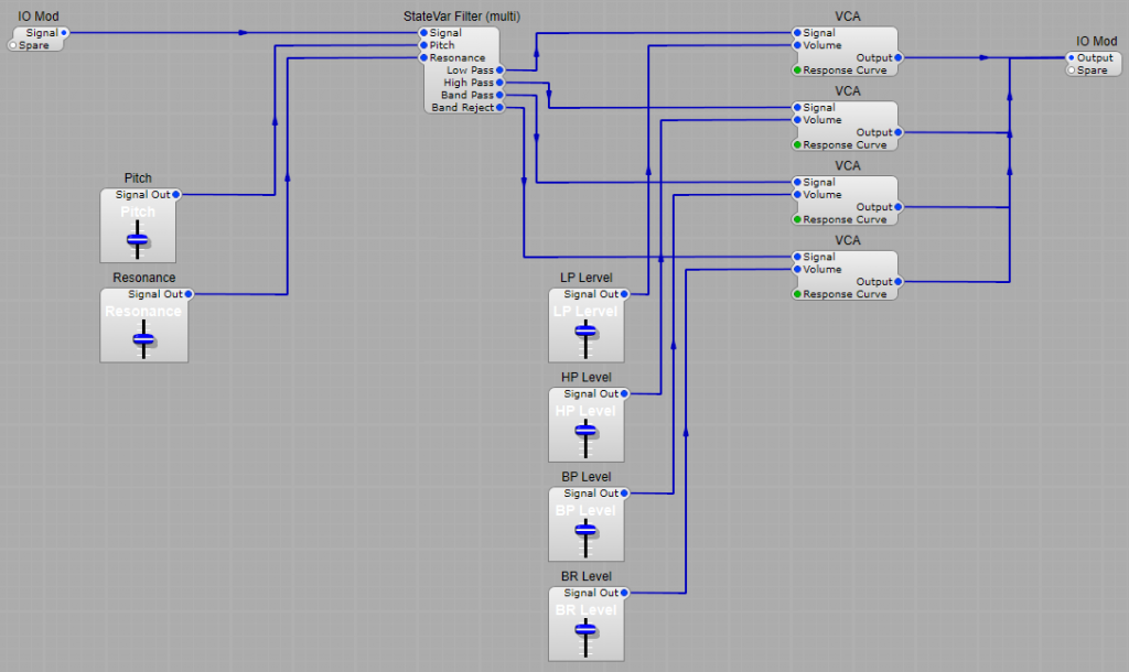
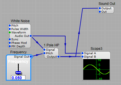
As the original LPG (Buchla) design had no resonance in it’s LPG mode I have just used two 1 Pole LP modules in series. There is no reason not to use an SVF or similar filter with resonance, but the aim here was to try and imitate the original design concept. If required you could use more filters to get a sharper Low Pass cut-off.
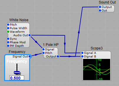
Here comes the strange bit (well I think it is), when used just as an LPF the module did have resonance, so for this mode there is an additional SVF in two stage Low Pass mode, wired up as a seperate filter that only operates in this (LPF) mode.

The VCA

Although we are using an exponential CV envelope for the VCA, I found contrary to what I first expected the results sounded better if the Response Curve is left at the default exponential setting.

Voltage offsets.

The voltage offsets shown are to compensate for the effect of the exponential voltage conversion modules, to restore the correct 0 volts level for the “off” portion of the envelopes. Likewise we need the Level Adj modules to reduce the envelope voltages to their normal 10 V maximum.
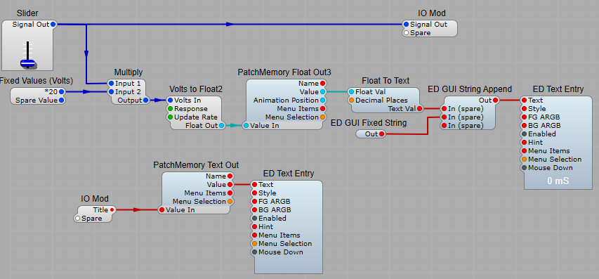
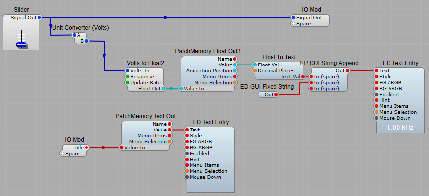
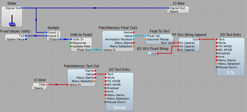
I used a fixed volts module to show the offset, gain and divisor values, and here’s a list of those values…
List of offset voltage values;
VCA Volume = -1V, (VCA Volume plug)
Filter Pitch = -1V, (1 Pole LP Pitch plug)
Divide by 2 = 2.5V (VCA Curve divider Input 2 plug)
Up Time /10 = 10V (Divider for ED Glider module)
Pulse Length dS = 0.1 (Monostable pulse length) Note: This offset is needed, if the Monostable Pulse Length is set to 0 it will not output any pulse at all.
Gain *01 = 0.1V LPF (Curve Level Adj module Input 2)
Curve 15 = 15 V (Divide Input 2 for VCA Curve) This affects how the initial decay curve of the exponential module feeding the VCA to imitate the differences in VACTROL characteristics.
Note: Feel free to experiment with some of these values, but do be aware that we are dealing with exponentials and small changes can mean a large increse in output…make small changes incrementally. Be careful of your monitors/headphones and your hearing.
Note: Changes in divide or gain module voltages will affect what voltage values you need on the LP Filter and VCA offsets.

Note: I have added a separate Output plug in this modification for the Low Pass Filter section, as this would need to be passed through a separate VCA anyway.

Auto filters.

22/05/2025 / Stephen / 0 Comments

An auto filter is like a standard VCF, but instead of controlling it with an LFO or ADSR, the filter frequency is controlled by an envelope (or Peak) follower.

The Peak Follower:

The peak follower detects the peak signal level of the audio input. This can then be applied to the pitch input of the VCF module.
The output attempts to follow the envelope (level) of the input signal.
The Attack and Decay control voltages can be converted from volts to milliseconds, this is calculated by multiplying by the voltage by 20. i.e. 1V = 20ms.
Both the Attack and Decay rates do change with frequency. The Peak Follower responds slower to Low frequencies, faster to high frequency signals. The formula above is calculated for a 1000 Hz sine wave. This is more or less how an analogue peak follower would behave in the real world.
Note: Very short decay times will mean that the Peak Follower won’t be following the real peak voltage, as it will start to follow the low frequency components of the signal rather than the peak audio level.

Adjusting the filter sweep.

This is quite simple, all we need to do is add a Level Adj module to the Signal Out plug of the Peak follower, with a slider control connected to input 2. There is no reason to stick to the Moog Filter for the audio filter, any type will do (as long as it’s a type that allows modulation of the pitch plug).

Set the controls…

Peak Attack/Decay sliders.
You’ll see that these controls don’t look exactly like the standard SE sliders would.
Yes, I have modified them. The Peak attack and decay sliders have the following structure:
The only points of note are;
1) Multiply module is used to convert from Volts to mS, just set the value on the Input 2 plug to 20.
2) Volts to Float 2, Response should be Volts DC (fast), update rate 10 Hz.
3) Float to Text, set decimal places to 0 (none), we really don’t need to be that accurate!
4) ED GUI String Append, the second input plug needs to have a space before the mS text to read neatly. With this module the first plug will be the main value, and each spare plug will be appended text.
5) The two “floating” modules PatchMemory Text Entry, and ED Text entry are used to display the title of the control slider.

Filter control (Pitch).
There’s a conversion module used here, so we can display the filter frequency in kHz. Just use the Unit Converter (Volts) module, with its mode set to Volts to kHz, and change the text on the ED GUI Fixed String to read kHz (don’t forget the space at the start of the text!).

Sweep and Resonance sliders.
These are the same as the Attack/Decay sliders with two changes;
1) Multiply, the Input 2 is set to 10, so that we change the readout from 0 to 10 to 0 to 100.
2) Change the text on the ED GUI Fixed String to %.

This is quite a versatile module, it can be used (as I have shown) as a VST filter sweep effect, or you could modify it to include in a Synthesizer.
You could also modify the filter to make it into an “Auto-Wah” effect for use with a guitar or other instrument.

Using the DAM Filter Draw module

30/04/2025 / Stephen / 0 Comments

Many thanks go to Davidson for his very handy range of SE modules.
This particular module allows us to have a visual representation of a filter’s frequency response, and to be able to control the cutoff and resonance from either the graphic display, or an external control voltage. I have used an SV filter in this project.

The DAM Filter Draw module.

Hint: The usual the text supplied to this plug will give you a pop up hint when the mouse is over the display window.
Menu Items/Selection: Used for the right click menu items and the choice made.
Mouse Down X:
Mouse Down Y:
Pos X Cut: Input/Output for the filter X value, which is connected to the filter’s Pitch or Frequency plug. Values are between 0-1 Floating, so when connecting to a Patch Memory always use the Animation Position plug.
Pos Y Reso: Input/Output for the filter Y value, which is connected to the filter’s Resonance, Q or Gain plug. Values are between 0-1 Floating, so when connecting to a Patch Memory always use the Animation Position plug.
Grasp Off/On: When this plug has the Boolean value of 1 (On, or True) you can adjust the parameters only by dragging the shape curve. When it has a Boolean value of 0 (Off, or False) you can adjust the Cut and Reso values by clicking or dragging anywhere in the display window.
Filter: You can set the filter mode for the display using the appropriate integer values; Low Pass=0,High Pass=1,Band Pass=2, Band Reject=3,Peak=4,Low Shelf=5,High Shelf=6,ST=7,CN=8
Note: ST allows you to drag the filter between Band Pass and Band Reject, CN gives a variable frequency, variable width Band Pass (I’m going to assume here that these options relate to a future filter release from Davidson?)
Slope: -12db (Single pole SV)=0, -24db/Octave (2 Pole SV)=1.
BG ARGB: Sets the background colour of the display window in the usual ARGB format. Hex codes won’t work here.
Line size: Sets the colour of the curve line in the usual ARGB format. Hex codes won’t work here.
Gradient Flip: You can invert the positions of the gradient colours using 0 or 1.
Fill Below/Above Center: Places the fill colours above or below the filter curve (although this is an integer plug there are only the two options). Below the curve = 0,
above the curve = 1.
Fill Top ARGB: Specify the upper portion of the gradient fill colour as ARGB (Not Hex, that won’t work)
Fill Bottom ARGB: Specify the upper portion of the gradient fill colour as ARGB (Not Hex, that won’t work)
Grid Off/On: 1 switches the centre grid on, 0 turns it off.
Grid Box Off/On: 1 switches the outer grid on, 0 turns it off.
Grid Line Size: Sets the thickness of the grid Note: this is a Floating point value not integer so you have a fine control over the grid thickness.
Grid ARGB: Specify the grid colour as ARGB (Not Hex, that won’t work)

Filter type options.

The Filter Draw module has more filter type options than we need but as the ones we are using are in the same sequence as the SV filter options this doesn’t matter. The unwanted options are just not used ( the drop down list is automatically taken from the SV filters options list).

Controlling the filter from the Filter Draw module.

This is done via the the two PatchMemory Float3 modules:
Pos X Cut controls the filter’s cutoff frequency
Pos Y Cut controls the filter’s resonance level.
These modules convert from GUI values to DSP, which is then converted from Float values to Voltage values for the Cutoff and Resonance plugs on the filter module, and convert the 0-1 Float range to the normal 0-10 V range for DSP controls.

CV Inputs.

Next we have two QTN_Volt2GUIFloat modules to take the external control voltages, and perform two functions 1) convert the incoming DSP voltage to GUI float, 2) redirect the output Float value to the left hand side of the module so it can be connected to the PatchMemory Value plug.
When this input voltage changes it will shift the appropriate x or y position on the Filter Draw module, and the related control value on the SV filter.

Filter Options.

As I said earlier we don’t need to set up any specially formatted lists, we can just use to PatchMemory List3 modules, and ED List Entry modules (OK you can use the stock ones, but I like Elena’s as you can set the background and text colours to suit your colour scheme).

Filters: FAQ’s and tips.

30/03/2025 / Stephen / 0 Comments

Float plugs.

I notice some filters have the lighter blue “Float” plugs? Synthedit allows me to connect a voltage to these plugs, but when I change the value quickly or modulate them the filter makes horrible crackling and clicking noises. What can I do to stop this? The short and simple answer is: Do not connect a Voltage to the Float plugs and do not modulate the values.
These values must never be changed rapidly. A filter that has it’s pitch controlled by a float value should not have the frequency changed rapidly.

Minimum filter frequency.

I connected up a filter so it has a range of 0 to 10 kHz, but the lowest frequency it will go to is about 14Hz? What am I doing wrong.
Nothing. All filters in Synthedit have a deliberately restricted frequency range.
Anyway, there is no such frequency as 0 Hz… if you think about it this means the voltage never changes, which means that it is really DC, so the only values that apply are Volts (in Synthedit we don’t need to consider Amps and Watts).

My filters go up to a certain frequency and no more.

This is intentional. The pitch control voltages on most (if not all) filters are internally clipped at 10 V. Often if you try to take the frequency of a DSP filter too high it will either; crash and stop working, make an awful noise, or exhibit strange behaviours. In any case when we are working with any form of digital signal there is that upper frequency limit set by our sample rate, the Nyquist Frequency where if we exceed this a lot of harsh distortion known as “aliasing” is produced.

SINC filters and dB/ Octave “roll off”.

The short answer to this question is for SINC filters no you cannot translate the “Taps” setting to dB/Octave. The number of Taps must also be an integer, hence the plug being an orange integer plug. (Just as in the “real” world you can’t have half a filter stage!).

The slope cannot be defined in dB/oct for windowed sinc FIR filters. Rather you should use transition bandwidth. There is no straightforward conversion of slope in dB/oct to transition bandwidth due to conceptual differences between FIR and IIR filters. IIR filters do not have a defined stopband.
https://eeglab.org/others/Firfilt_FAQ.html

There is no SINC bandpass filter, can I make one?

Yes by cascading an HPF and an LPF in series you can get a bandpass filter, and by having an LPF and HPF in parallel you’ll get a notch filter. Altering the number of Taps will change the notch or pass band shape, and changing the frequencies will change their width or Q. Note: For the notch filter the number of TAPS must be kept the same in both filters for it to work correctly, otherwise latency can affect the filter operation.

SINC Filter Latency.

Although there are no concerns about frequency dependent phase shift with a SINC filter there is latency which relates only to the number of TAPS, You can see below that the initial pulse from the oscillator (green), has been significantly delayed by passing through the filter with the number of TAPS set to 171.

Changing the filter frequency from 14 kHz (see above) down to 8 kHz (see below) only changes the pulse shape and amplitude, not the delay time.

Note: By setting Delay Compensation to Full in the preferences dialogue, the effects of latency will be removed.

The effects of enabling Delay Compensation (see below).

Notice also the ringing or ripple effect around the output pulses from the filter, this is a normal artefact with SINC filters with high sample rates (above 44kHz) and like latency is dependent on the number of TAPS, not filter frequency (the input signal does seem to affect this ripple effect though).

Can I “see” the frequency spectrum of a filter?

Yes there is a handy module available the Freq Analyser2, connect up a white noise source (the best signal for doing this since it contains the whole of the audio frequency spectrum). All these filters have the same cutoff frequency so you can see the difference in how they attenuate the frequencies outside the passband, and in the Moog filter the resonant peak it creates.

FIR FILTERS. (Finite Impulse Response)

The SINC Lowpass is a linear-phase FIR Filter. “Taps” specifies the number of coefficients, more taps gives us a steeper cutoff response, but introduces progressively more latency.
FIR filters don’t have poles only zeros : poles mean ‘feedback’ and once there is feedback it is an IIR filter.
The SINC Lowpass filter has latency, for example if you send an impulse into it, you can see it emerge a little later in time…
FIR Filters do not introduce phase shift, however they do introduce latency. This is dependent on the number of poles, and is frequency independent.
The latency is always in integer steps.
You can consider all FIR filters to be a multitap delay with no feedback, with all the taps spaced 1 sample apart, gain is then applied per tap and then all taps are added together.
So for a 171 tap delay, you have 170 delays, 171 gains (like level adjust modules) and 170 adds.

List of FIR filters in SynthEdit;

Filters built into SE’s Oversampling modules.
SINC High pass filters,
SINC Low pass filters.

IIR Filters (Infinite Impulse Response).

The output of IIR filters as they decay (in theory) never stops changing, and will never reach zero. The output just gets closer and closer to zero forever.
For this reason the 1-pole filters in SE will assume that when the filter’s output drops below a certain point that it is ‘near enough to zero’ and it’s the right point for the Filter to “sleep”.
Phase shift.
Phase shift in IIR filters (as in the physical analogue equivalents) is frequency dependent. Every IIR filter introduces some per-frequency phase shift.
Cascading filters will obviously sum all of the phase shifts.
Limits to parameters.
For all filters, your filter cutoff can never be 0 Hz or Nyquist (we are subject to the laws of physics, maths, and electronics), so if they are intended to be modulated to the extremes of that range, then we have to clip the cutoff frequency, and the Q (feedback/resonance) to ranges that don’t exceed the valid ranges.
Biquad Filters.
Because Biquads are unstable at low frequencies, a clip value of 5 to 10 Hertz, keeps things under control, and that’s out of the range of human hearing anyway.
Butterworth Filters.
These filters are intended to be preset to a particular frequency, and not have the frequency changed whilst in use. They will not perform well if the frequency is changed whilst the VST is running. They are designed for tone controls and equalization usage. They have a very flat frequency response and so make excellent tone controls.
If you really need a bandpass filter that can have it’s frequency changed always use an SV filter, you can fix the resonance at 0, and if you need a narrower pass-band cascade the filters (beware of phase shift if you are mixing wet and dry audio though), but you would get phase changes with the Butterworth EQ filters anyway!

List of IIR Filters;
1 Pole LPF
1 Pole HPF
Butterworth
Biquad
Moog ladder filters
SV Filters
All Pass filters
Hilbert or “Dome/Bode” filters
Steiner Parker
Claudia’s Filter module
The “Panda” filter.
….Just about all the Synthedit stock and third party filters in fact.

Parallel Filtering

27/02/2025 / Stephen / 0 Comments

The title says most of it really. We can take a single sound source and split it to feed two filters which are independent of each other (separate controls and modulation inputs). You can use this to provide a “pseudo stereo” effect where the left and right channels have different filtering. Low pass on the left, and high pass on the right. Different polarities and rates of modulation can create some interesting stereo swirling and rotation style effects. Of course there is no need to have both filters fed by the same sound source, if you want they can be two different sound sources. You can mix and match types of filter too. There’s no reason why you should not have a Moog low pass in the left, and a State Variable in the right channel.

VCF with multiple outputs

27/02/2025 / Stephen / 0 Comments

Using one of the StateVar Filter (Multi) can give us a very wide range of filtering options by mixing the outputs to combine their different characteristics in a number of ways.

Simple Low Pass filtering

Combining Low pass and Band Reject filtering.

Note how in this example we get both a notch and a strong resonant peak.

Combining High Pass and Band Reject filtering.

Note in the HP/BR example the peak has now moved higher than the notch frequency.

Combining Low, High and Band pass.

We now get a strong resonant peak giving a frequency boost, but not much in the way of any filtering out of frequencies.

A two mode alternative to the four mode filter.

This model uses the same filter, but we only use the Low and High pass outputs. The Low pass is fed directly to one input of the X-Mix module, whilst the High pass has the option of being fed through an inverter. The inverter affects the output frequency spectrum.
This is similar to those wonderful Oberheim Expander filters where you could cross mix the High and Low pass outputs. It won’t sound quite the same due to the chips that Oberheim filters used, but close to them.

High Pass in phase.

The frequency spectrum is fairly flat when HP and LP are in balance with no obvious resonant peak. Whereas below in the first example once the High Pass starts to predominate we get a notch with the resonant peak at a higher frequency.

And in this example where the Low Pass is starting to predominate we get a notch with the resonant peak at a lower frequency.

High pass out of phase.

By inverting the high pass output, we can create a strong resonant peak when both High and Low pass signals are in balance, whereas in the previous example where the High pass was not inverted the output is almost flat when the two signals are in balance.

Filters and Phase Shift.

12/02/2025 / Stephen / 0 Comments

All filters in Synthedit will by their nature exhibit some phase shift at some point in their frequency spectrum. Some filters exhibit more phase shift than others.
(Even analogue filters will introduce phase shift)

Phase shift and Analogue filters.

A basic analogue resistor–capacitor (RC) low-pass filter, as an example, will shift the output sine wave by up to 90° compared to the input sine wave. The “up to” is important—the actual phase shift generated in the circuit also depends on the frequency of the signal passing through the filter. As you can see this quickly becomes a complex subject.

Moog filters and phase shift.

A Moog ladder filter, introduces a significant phase shift as the signal frequency approaches the filter cutoff frequency, with each stage of the filter adding about 45 degrees of phase shift, which gives us a total phase shift of nearly 180 degrees at the cutoff frequency for a typical 4-stage Moog filter; it is this phase shift that contributes to the unique “warm” and resonant sound of Moog synthesizers when filtering sounds at, or near to the cutoff frequency.

SV Filters and phase shift.

An SV filter, which stands for “State Variable Filter,” introduces phase shift by design, meaning it alters the timing of different frequency components within a signal as it filters them, with the amount of phase shift varying depending on the frequency and filter settings; (this is a common to most filters, not just SV filters), but the design of an SV filter can make this phase shift far more pronounced at certain frequencies.
Key points about SV filters and phase shift:
The phase shift in an SV filter arises from the internal circuitry and the way it interacts with different frequencies, causing different time delays for various components of the signal.
The Impact on the filtered sound:
When filtering audio with an SV filter, a very noticeable phase shift can manifest as subtle changes in the sound quality, particularly affecting the timing of transients or the overall “naturalness” of the filtered sound.

“Korg MS20” filters, otherwise known as Sallen-Key filters.

The Sallen-Key filter, is a second-order active filter, with a phase shift that approaches -90 degrees at its cut-off frequency, with its phase response smoothly transitioning from 0 degrees at lower frequencies to -180 degrees at very high frequencies.
Its key characteristics include:
1) High input impedance,
2) Low output impedance,
3) Good stability, with the ability to readily adjust its cut-off frequency and quality factor (Q) by adjusting the values of its resistors and capacitors, allowing for a flexible filter design.
The Sallen-Key design used in the Korg MS20 also had the ability to go into saturation giving some unique “screaming” sounds.

Summary.
As you can see phase shift in filters is normal, and is inherent in their design and the resulting unique “flavour” imparted to the output filtered sounds. Without their built in phase response there would be no “Moog filter” sound.

Digital filters.

Most filters exhibit a phase shift of some sort, with DSP the shift is always in the form of a small delay in the signal due to the large number of complex calculations. The more efficient the computation method used, the lower the degree of phase shift introduced by the filter, unless phase shift is called for to recreate (for example) the sound of a Moog ladder filter.

For a simple 1-pole hp filter, the phase response at the cut-off frequency will be about 45 deg. As a general rule the lower the number of poles in the filter, the less the phase shift will be. All of the filters in Synthedit will introduce some degree of phase shift, this is largely unavoidable.
The degree of phase shift is dependent on the type of filter, number of poles or steepness of cutoff slope.

You can see below the phase shift that even a simple 1 pole HP filter introduces:
At 50 Hz, the two ‘scope traces are superimposed- we have an almost zero phase shift between input and output.

However at 500 Hz you can see there is a marked shift in phase (Ignoring the difference in amplitude) between the input and output signals.

Cumulative phase shift.

If you cascade (or stack) filters the phase shift is also cumulative (adds up), so if one filter gave you 45 degrees at 1kHz, two filters will give you 90 degrees phase shift at 1 kHz.

Why and when is phase shift important?

Often you wouldn’t notice that a filter was introducing phase shift, however it soon becomes apparent when you mix the filtered signal with the original “dry” signal. As the filter frequency changes you would likely notice a “phasing” effect on the sound in addition to any timbral changes from the filter itself.
You can see this in the sequence of screenshots below:

100% Low pass Moog filter.

With a mix of 50% Low pass and 50% dry signal, you can see there is a pronounced notch at 2kHz.

And with 100% dry signal we get a more or less flat white noise spectrum.

Introducing feedback (resonance) into the filter introduces further phase shifting effects as raising and lowering the resonance level will alter the phase shift quite markedly at mid range filter frequencies.

0 Resonance at a middle range frequency gives this pronounced phase shift.

Whereas with a resonance of 8.3 the signals are approaching being in phase again.

As you can see phase shift in filters is not a simple and easily predictable subject.

The only filters that I have tested in Synthedit to give a constant phase shift over their frequency range are the high and low pass SINC filters.

SINC (IIR) Filters

18/07/2024 / Stephen / 0 Comments

Windowed-sinc filters are used to separate one band of frequencies from another. They are very stable, produce few surprises, and can be pushed to incredible performance levels.
These exceptional frequency cutoff characteristics are obtained at the expense of poor performance in: a) the time domain (meaning they will always introduce latency), b) excessive ripple and c) overshoot in the step response.
In the image below you can see how the signal pulse (Oscillator 280Hz) is delayed as the number of “Taps” at a filter frequency of 5 kHz increases, and the amount of “ringing” or ripple on the pulse waveform also increases.

Increasing TAPs increases the latency:

TAPs and latency.

The SINC Lowpass filter is a linear-phase FIR Filter. The number of “taps” specifies the number of coefficients, more TAPs means increased filter cut-off steepness as seen below however, increasing the number of TAPs introduces more latency. In SynthEdit however there is latency compensation. The module is watching for any change to the default value of the ‘Taps’ pin. The module then uses this value to calculate how much latency compensation it requires and passes that value to the host via the ‘SetLatency’ method. Latency is measured in sample frames.
The module reports this latency to SynthEdit to enable PDC (Plugin Delay Compensation). PDC hides the effect of latency through the clever use of delay lines. You can literally think of all FIR/SINC filters as a multitap delay with no feedback, all the taps are spaced 1 sample apart, then gain is applied per tap and then all taps are added together. So for a 171 tap delay, you have 170 delays, 171 gains (like level adjust modules) and 170 adds. It’s already well optimised with SSE2, as it’s doing 4 calculations at a time.

Resonance/Q/Feedback.

SINC filters do not include a feedback path, so have no feedback, resonance, or “Q” control plug. The are intended to be used as a filter with a very steep low/high pass cutoff characteristic, rather than for colouration of sound.

Increasing the number of TAPs and the effect on frequency roll-off.

Note about 0 Hz filter cut-off:

Although this filter will allow you to set a cut-off frequency of 0 Hz, you cannot use a filter frequency of 0Hz, this is is an ‘illegal‘ value. You will get quite loud clicks and pops, along with “glitching”.
Most SynthEdit filters are “clipped” internally so that end-users don’t input wrong values (this comes at a slight CPU cost of course), usually limited to just above 0Hz and just below the Nyquist frequency.
Why 0Hz is illegal is easiest to explain with a simple 6dB/Octave lowpass. If we set the lowpass to 100Hz, then 200Hz (2nd octave) will be filtered by -6dB, 300Hz (3rd Octave) by -12dB, 400Hz(4th Octave) by -18dB and so on, hence the “6dB/Octave” name. Now try and do the same thing with 0Hz….what is an octave above 0? 0 multiplied by 0 is still 0. It’s the same as dividing by zero.
To prevent loud pops, clicks and glitching you must limit the lowest cut-off frequency to 14 Hz.
Just be sure to limit your patch memory values to prevent illegal values.
Other than this the SINC filters are suitable for fast modulation of the cut-off frequency. Note that there is no resonance/feedback on these filters.

Changing TAP value.

One point to note with SINC filters is that when you change the TAP value the audio engine has to reset for the recalculation process.

TAP Value and filter cut-off slope.

Although we can vary the cutoff slope on SINC filters by altering the TAP number, this bears no relation to the more familiar dB/Octave slope, so unfortunately you cannot say that a certain TAP number is equivalent to a particular dB/Octave cutoff slope. This is due to the DSP structure, and the way these filters work, they are a using a different method of filtering which bears little or no mathematical resemblance to the more traditional analogue filter emulations.

Some other Useful filters in the TD range of Modules.

18/02/2024 / Stephen / 3 Comments

Butterworth filters.

TD_Butterworth_HP
Type: Butterworth high pass filter.
Can be set from 2nd order filtering to 12th order filtering.
There is no internal clipping on the kHz input voltage, and the control voltage only has the 1V/kHz characteristic.

TD_Butterworth_LP
Type: Butterworth low pass filter.
Can be set from 2nd order filtering to 12th order filtering.
There is no internal clipping on the kHz input voltage, and the control voltage only has the 1V/kHz characteristic.

TD_P1Z1
Type: 1 Pole (6dB per octave), 1 Zero Filter.
A specific design of Butterworth filter.
Selectable filter modes: Low Pass, High Pass, Bandpass.

TD_P1Z1_ST
Type: Stereo version of the 1 Pole (6dB per octave), 1 Zero Filter.
A specific design of Butterworth filter.
Selectable filter modes: Low Pass, High Pass, Bandpass.

State Variable Filters.

TD_SV2
Type: Linear State Variable Filter
Filter Modes; Low pass 12dB per octave, High pass 12dB per octave, Bandpass 6dB per octave, Band reject 6dB per octave, Low pass 6dB per octave,
High pass 6 dB per octave, All pass 12dB per octave.

TD_SV2_ST
Type: Stereo Linear State Variable Filter
Filter Modes; Low pass 12dB per octave, High pass 12dB per octave, Bandpass 6dB per octave, Band reject 6dB per octave, Low pass 6dB per octave,
High pass 6 dB per octave, All pass 12dB per octave.

State Variable Formant filters.

TD_SVX4
Four zero peak gain state variable bandpass filters internally connected in parallel.
Notes: Primarily designed as a building block for designers to create their own formant filters. Having a quad filter module uses less CPU than individual filters.

TD_SVX4_ST
Stereo version. Four zero peak gain state variable bandpass filters internally connected in parallel.

Audio Crossover Filters.

TD_Xover12
Type: 12dB per octave crossover filter.
This is module is built out of a standard State Variable filter and is suitable for modulation if need be

TD_Xover12_ST
Stereo 12dB per octave crossover filter.
This is module is built out of a standard State Variable filter and is suitable for modulation if need be.

Hilbert 90 degree filter network.

TD_Hilbert_A
Type: Hilbert Filter network, this network creates 90 degrees phase difference between the two outputs.
Notes: This uses an IIR 2 x 8 pole 90 degree phase-difference network. The outputs are approximately 90 degrees apart in phase, which is needed to build frequency shifters. The approximation in phase shift is not a problem for frequency shifting in general because if the input frequency shifts, so does it’s ability to cancel out with the original signal.

TD_Slew2
Control signal “slewer”.
The type of slew can be set to; Constant rate, Constant time.
Notes on Constant Time: It takes the same amount of time to go from 0-1 or 0-10. 1 volt = 1 second. The curve is exponential.
Volts slew time is limited to a maximum of 20 seconds and a minimum of 1 millisecond.
Notes on Constant Rate: It takes less time to go from 0-1 than 0-10, as it moves at the same speed between points. 1volt per 1second. The curve is linear.
Volts slew rate is limited to a maximum of 20,000 volt per second and a minimum of 0.1 volt per second.
Useful for introducing “glide/portamento” effects for control voltages, removing “stepper” effects, and smoothing out the output of sample/hold generators.

TD_PeakHold
Type: Peak Hold Filter
Notes: Generally used as a Peak hold for GUIs, and is not recommended for audio use. (You need to use a DSP-GUI bridge or Patch Mem)

TD_PeakHold
Type: Stereo Peak Hold Filter
Notes: Generally used as a Peak hold for GUIs, and is not recommended for audio use. (You need to use a DSP-GUI bridge or Patch Mem)

The TD range of Synthesizer filters.

18/02/2024 / Stephen / 0 Comments

These filters are all suitable for use as a Voltage Controlled Filter (VCF) in synthesizers, and as such can have their cutoff and resonance frequencies modulated rapidly.
Notes: It should be taken as read that all these filters have their control voltage internally limited to +10 Volts, and that they operate within the normalizer SynthEdit audio voltage range. Some may have the audio internally clipped so will distort at high input levels.

Ladder Filters.

TD_DiodeLP24_A
Type: 24dB per Octave frequency roll-off diode ladder lowpass filter type A
Notes: A simplified 4 pole diode-ladder lowpass filter with a single symmetrical non-linearity. Partial passband gain-loss compensation. Diode-ladder filters are unbuffered which leads to the cutoff frequency being a product of cutoff amount, input level and resonance.

TD_DiodeLP24_B
Type: 24dB per Octave frequency roll-off diode ladder Lowpass Filter Type B
Notes: A 4 pole diode-ladder lowpass filter, the first pole is an octave higher, with an additional unbuffered high pass filter in the feedback path that partially damps the resonance at low cut-off frequencies.
An extra buffered high pass filter is on the input too. So it is more like a 5 pole + 1 pole filter. The filter cutoff slope is not a constant vs frequency. There are asymmetrical non-linearities, and partial passband gain-loss compensation. Diode-ladder filters are unbuffered which lead to the cutoff frequency being a product of cutoff amount, input level and resonance. Because of the first pole being an octave higher, maximum cutoff is 9.5 Octaves (~9.95kHz) if the sample rate is equal or less than 48kHz, 10.5 octaves (~19.9kHz) otherwise.

TD_DiodeLP24_C (EMS VCS3 Emulation)
Type: 24dB per Octave frequency roll-off diode ladder Lowpass Filter Type C
Notes: A 4 pole diode-ladder lowpass filter inspired by the paper “Efficient polynomial implementation of the EMS VCS3 filter” by Stefano Zambon and Federico Fontana. However it uses ‘Mystan’s Pivot’ method to approximate the non-linearities instead, which in this case are asymmetrical. Full passband gain-loss compensation. Diode-ladder filters are unbuffered which lead to the cutoff frequency being a product of cutoff amount, input level and resonance.

TD_Ladder5out_HP
Type: Linear 4 pole High pass filter with five outputs
Note: This module is useful as the basis for pole-mixing filters.
Note: The filter does not self oscillate.
Traditionally, 4-pole pole-mixing filters only mix the 4 poles.
Two of the poles are inverting – either 1 and 3 or 2 and 4. Some short/set-high/bypass the first pole under some circumstances to get more variations.
With this version, instead of bypassing – all you have to do is move the mixing-coefficients up i.e. hp1 coefficient, hp2 coefficient, hp3 coefficient becomes in-hp4 coefficient, hp1 coefficient, hp2 coefficient.

TD_Ladder5out_LP
Type: Linear 4 pole Lowpass Filter with 5 outputs
Notes: This module is useful as the basis for pole-mixing filters.
Note: The filter does not self oscillate.
Traditionally, 4-pole pole-mixing filters only mix the 4 poles.
Two of the poles are inverting – either 1 and 3 or 2 and 4. Some short/set-high/bypass the first pole under some circumstances to get more variations.
With this version, instead of bypassing – all you have to do is move the mixing-coefficients up i.e. lp1 coefficient, lp2 coefficient, lp3 coefficient becomes in-lp4 coefficient, lp1 coefficient, lp2 coefficient.

TD_LadderHP24_A
Type: 24dB/Octave Transistor-Ladder High pass Filter
Asymmetrical non-linearities. Partial passband gain-loss compensation. Self oscillates.

TD_LadderLP18_A
Type: 18dB per Octave Transistor-Ladder Lowpass Filter
Simplified filter version with a single symmetrical non-linearity. No passband gain-loss compensation. Self oscillates.

TD_LadderLP24_A
Type: 24dB/Octave Transistor-Ladder Lowpass Filter Type A
Simplified version with a single asymmetrical non-linearity. No passband gain-loss compensation (classic behaviour). Self oscillates.

TD_LadderLP24_B
Type: 24dB per Octave Transistor-Ladder Lowpass Filter Type B
Multiple asymmetrical non-linearities. Partial passband gain-loss compensation. Note: The filter does not self-oscillate.

TD_LadderLP24_C
Type: 24dB/Octave Transistor-Ladder Lowpass Filter Type C
This filter has a buffered high pass filter in the feedback path. This prevents self oscillation at very low frequencies and also prevents bass loss at high resonance levels. Asymmetrical non-linearities.

Oberheim X-Pander type filter.

TD_Panda (Inspired by the Oberheim X-Pander filter)
Type: 4pole OTA Inspired Filter
Notes: The filter poles are mixed internally to create 25 different frequency responses. Produces predominantly 3rd harmonic distortion. Self oscillates.
List of Filter frequency responses; LP4, LP3, LP2, LP1, HP4, HP3, HP2, HP1, BP4, BP2, BPS, HP3LP1, HP2LP1, HP1LP3, HP1LP2, HP1BR2, BR2LP2, BR2LP1, BR4, BR2, BRBP2, LP1BR2HP1, LP1PK2, BR2PK2, HPX.

Sallen-Key filters.

TD_SK3P
Type: Buffered 12dB/Octave Lowpass Sallen-Key Filter
Frequency cutoff 12dB per octave slope. The extra pole is in the feedback path and limits resonance at higher frequencies and alters tracking a bit. Self-resonates up to about 3.7kHz. Symmetrical non-linearities.

TD_SK4P
Type: 12dB/Octave Lowpass Sallen-Key Filter
Experimental, has extra poles. Asymmetrical non-linearities.

TD_SK_A
Type: Multi-Mode Sallen-Key Filter; Low Pass 12dB per Octave, High Pass 6dB per Octave, Band Pass 6dB per Oct.
Buffered. This saves some CPU cycles compared to the Steiner modules. Asymmetrical non-linearity.

Steiner-Parker filters.

TD_Steiner_A
Type: Buffered Steiner-Parker multi-mode filter Type A
A Steiner-Parker filter is simply a multi-input Sallen-Key filter.
Symmetrical non-linearities. Does not self-oscillate. Maximum input is +/- 10 volts. If the sample rate is less than, or equal to 48 kHz, then the maximum cutoff frequency is approximately 14 kHz otherwise it is approximately 19.9kHz.

TD_Steiner_B
Type: Steiner-Parker Filter Type B
An unbuffered version of a Steiner-Parker filter (the feedback loop is still buffered), which simply is a multi-input Sallen-Key filter.
Asymmetrical non-linearities. Does not self-oscillate. Resonance decreases in higher octaves. Maximum input is +/- 10 volts.
If the the sample rate is less or equal to 48kHz, maximum cutoff frequency is approximately 17.3 kHz otherwise it is approximately 19.9 kHz.

TD_Steiner_C
Type: Steiner-Parker Filter Type C
A buffered version of a Steiner-Parker filter, which simply is a multi-input Sallen-Key filter. Bright asymmetrical non-linearities. Self-oscillates.
If the sample rate is less or equal to 48kHz, the maximum cutoff frequency is approximately 17.3kHz otherwise it is approximately 19.9kHz.

State-Variable filters.

TD_SV24_A
Type: Cascaded State Variable Filters Type A; 24dB per Octave Low pass, 24dB per Octave High pass, and 12dB per Octave Band pass.
Induced passband gain-loss to prevent too high levels with high resonance.
This is a non-linear filter but it is not able to self-oscillate.
This module uses less CPU than if two standard SE SV filters were cascaded.

TD_SV24_B
Type: Cascaded State Variable Filters Type B; 24dB per Octave Low pass, 24dB per Octave High pass, 12dB per Octave Band pass.
Induced passband gain-loss to prevent signal levels becoming too high with high levels of filter resonance.
This is non-linear filter but it is not able to self-oscillate. The resonance level decreases as the filter cutoff frequency increases.
This module uses less CPU than if two standard SE SV filters were cascaded.

TD_SV_C
Type: State Variable Filter Type C; 12dB per Octave Low pass, 6dB per Octave Band pass.
Experimental State Variable Filter that is modified by adding an extra feedback path around the structure, so it’s not really a true SV filter any more. Resonance decreases at higher frequencies. Asymmetrical non-linearities. Does not self oscillate.

TD_SVmo2
Type: Multiple Output State Variable Filter; 12dB/Octave Low pass, 6dB/Octave Band pass, 12dB/Octave High Pass
The filter outputs can be mixed, combined or otherwise processed to achieve other filter shapes. Non-linear filter.

TD_SVmo2_ST
Type: Stereo Multiple Output State Variable Filter 12dB/Octave Low pass, 6dB/Octave Band pass, 12dB/Octave High Pass
The filter outputs can be mixed, combined or otherwise processed to achieve other filter shapes. Non-linear filter.

TD_SVxfade
Type: Cross-fading State Variable Filter. Three pre-programmed selectable crossfade sequences.
Select the filter type and cross-fade sequence from;
Low pass /Band Reject /High pass,
Low pass /Peak /High pass,
Low pass /All pass /High pass.
The cross-fade voltage range is from -5 Volts to +5 Volts.

About Low Pass Gates (LPG).

Generating the attack/decay envelope.

LPF Curve and VCA Curve.

The filters

The VCA

Voltage offsets.

Related posts:

The Peak Follower:

Adjusting the filter sweep.

Set the controls…

Related posts:

The DAM Filter Draw module.

Filter type options.

Controlling the filter from the Filter Draw module.

CV Inputs.

Filter Options.

Related posts:

Float plugs.

Minimum filter frequency.

My filters go up to a certain frequency and no more.

SINC filters and dB/ Octave “roll off”.

There is no SINC bandpass filter, can I make one?

SINC Filter Latency.

Can I “see” the frequency spectrum of a filter?

FIR FILTERS. (Finite Impulse Response)

List of FIR filters in SynthEdit;

IIR Filters (Infinite Impulse Response).

Related posts:

Related posts:

Simple Low Pass filtering

Combining Low pass and Band Reject filtering.

Combining High Pass and Band Reject filtering.

Combining Low, High and Band pass.

A two mode alternative to the four mode filter.

High Pass in phase.

High pass out of phase.

Related posts:

Phase shift and Analogue filters.

Moog filters and phase shift.

SV Filters and phase shift.

“Korg MS20” filters, otherwise known as Sallen-Key filters.

Digital filters.

Cumulative phase shift.

Why and when is phase shift important?

Related posts:

TAPs and latency.

Resonance/Q/Feedback.

Note about 0 Hz filter cut-off:

Changing TAP value.

TAP Value and filter cut-off slope.

Related posts:

Butterworth filters.

State Variable Filters.

State Variable Formant filters.

Hilbert 90 degree filter network.

Related posts:

Ladder Filters.

Oberheim X-Pander type filter.

Sallen-Key filters.

Steiner-Parker filters.

State-Variable filters.

Related posts:

Recent Posts

Archives

Categories